

[In the summer of 2026, I had the opportunity to conduct research in the Khare Laboratory at Rutgers University under the mentorship of Dr. Sagar Khare and Austin Seamann. The Khare Lab is part of the Institute for Quantitative Biomedicine (IQB), and Dr. Khare is a Professor in the Department of Chemistry and Chemical Biology. My project focused on using AI-based protein design tools to design a binder for a photoswitchable protein. Below is a summary of the research, methods, and key outcomes from the project.]
Previous in the series: Designing Sequences While Preserving Diversity
Selecting 27 candidates from the final computational stage and generating predicted models
In the previous post I explained how we generated sequence-based designs while preserving structural and positional diversity. Here I will explain the final major stage of our pipeline in which we evaluated the remaining models and selected the final designs. We used AlphaFold3 to predict structures from the remaining 107 sequences and to evaluate how well the predicted binders matched the intended designs. We ran the model in two ways: (1) Chain B alone and (2) Chains A and B together. The Chain B-only run helped us examine the binder by itself, while the combined run allowed us to evaluate the binder-target complex (Fig. 1).
AlphaFold3 evaluated each binder alone and as part of the binder-target complex
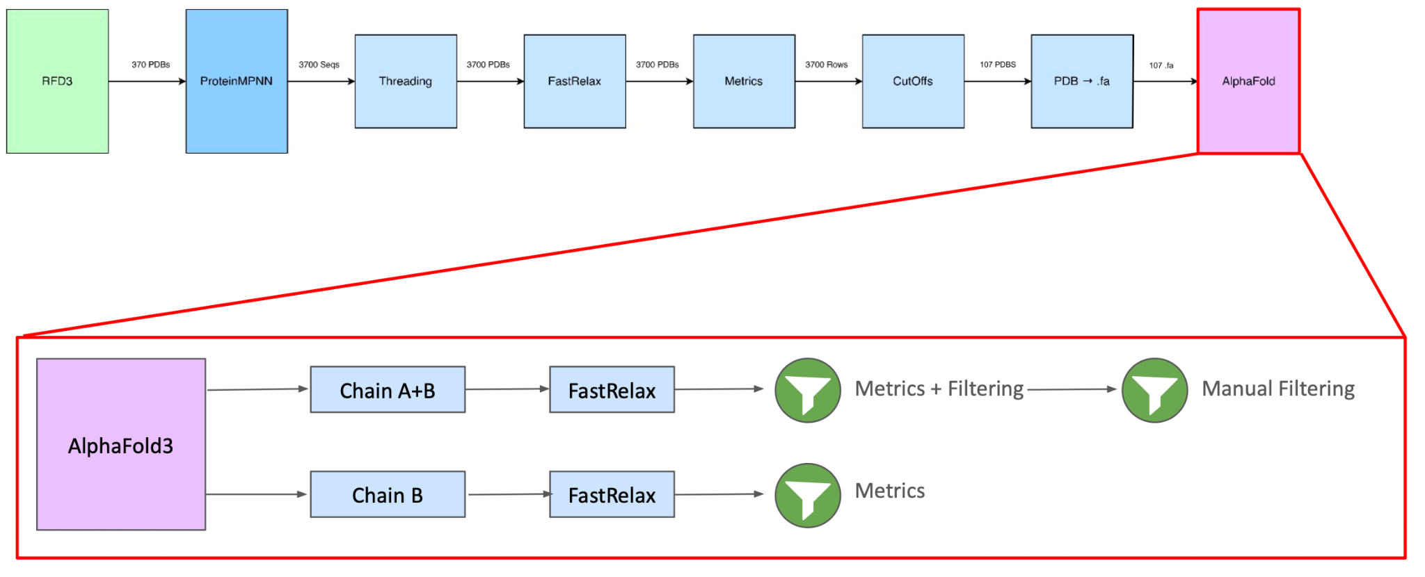
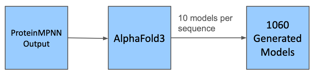
For each ProteinMPNN sequence, we generated about 10 AlphaFold3 models (Fig. 2). At this point, the slide reports a total of 1,060 generated models. After prediction, we processed the structures through FastRelax, metric calculations, filtering, and a manual review.
AlphaFold3 produced about 10 predicted models per designed sequence
After prediction, the structures went through FastRelax, metric calculations, filtering, and manual review.
Comparing predicted and intended structures
In this filter step, for each model we used the RMSD to compare the AlphaFold3 result with the earlier designed structure after alignment to Chain A (Fig. 3). The cutoff depended on the binder’s secondary structure, to allow beta-rich models slightly more flexibility:
· Alpha-rich designs needed an RMSD below 5.6 angstroms
· Beta-rich designs needed an RMSD below 6.5 angstroms
We observed that models with lower RMSD values more closely matched the earlier designs under this comparison. Therefore, models with high values were rejected.
RMSD filtering measured how closely AlphaFold3 predictions matched the intended binder-target structures
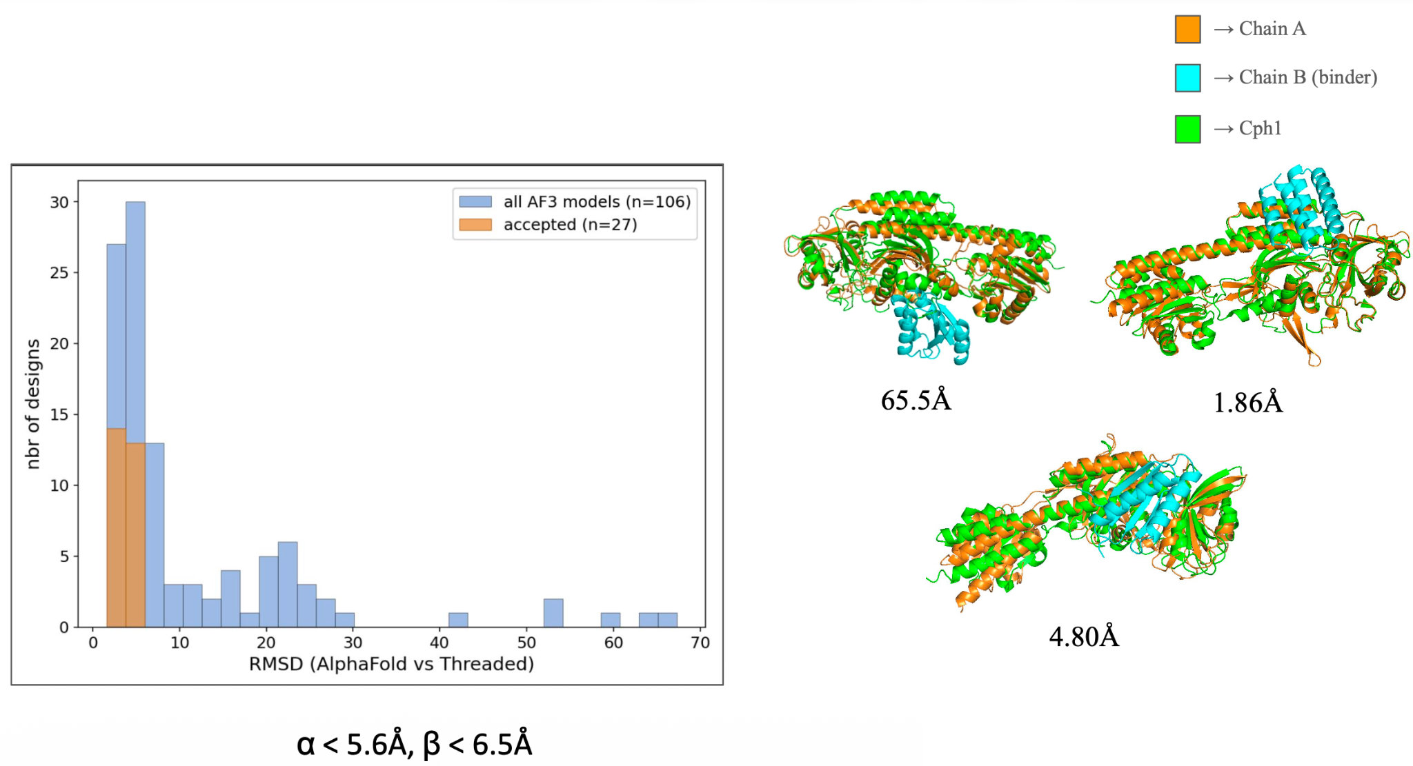
Models with lower RMSD values more closely matched the earlier designs under this comparison. Models with high values were rejected.
Measuring contacts with Chain A and Checking compactness again
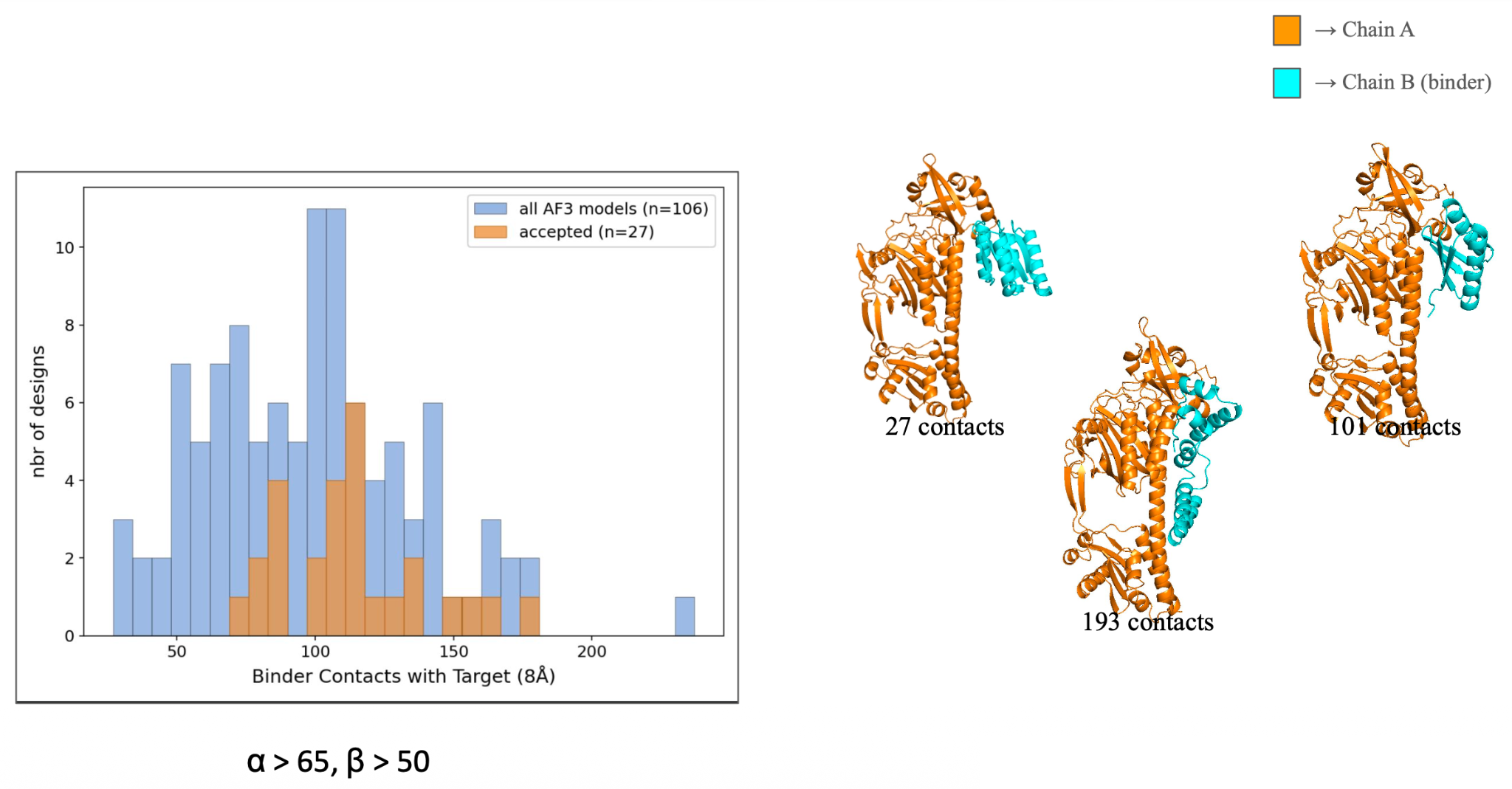
We also measured how many contacts the binder formed with Chain A. Alpha-rich designs needed more than 65 contacts, while beta-rich designs needed more than 50 (Fig. 4). Under the project’s filtering rules, we determined that a design with too few contacts did not interact with enough of the target surface.
The final filters required alpha-rich and beta-rich binders to form a minimum number of contacts with Chain A
Checking compactness again
Radius of gyration remained important during the AlphaFold3 stage. At this stage of the process, we determined the accepted range as 11.3 to 13.5 angstroms (Fig. 5). This check helped confirm that the predicted binder remained within the desired compact range after sequence design and structure prediction. The final-stage cutoff table also included dG/dSASA, helix length, beta-sheet length, clashes, and loop percentage.
The final radius-of-gyration filter kept predicted binders between 11.3 and 13.5 angstroms
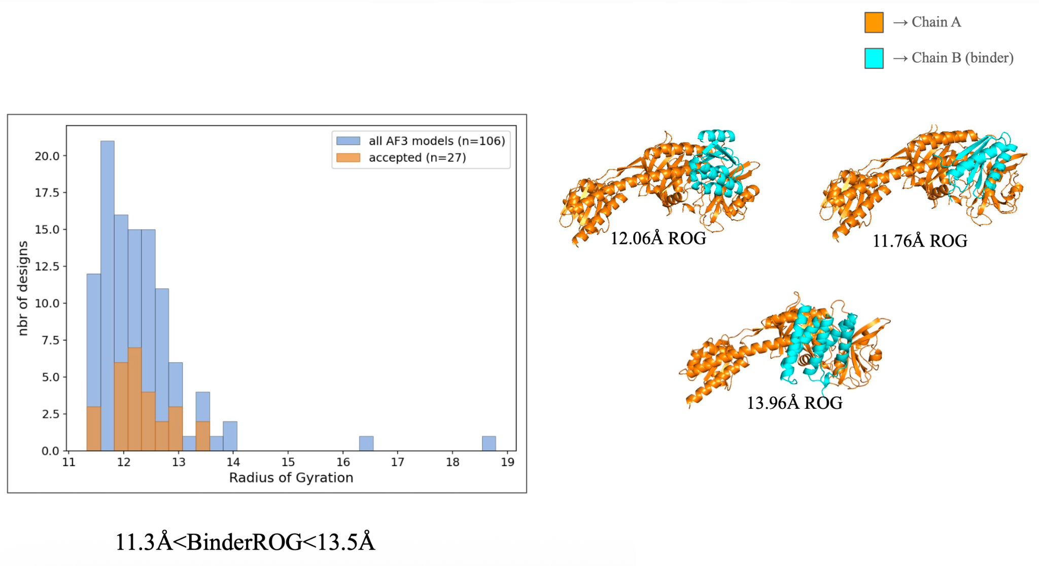
The final-stage cutoff table also included dG/dSASA, helix length, beta-sheet length, clashes, and loop percentage.
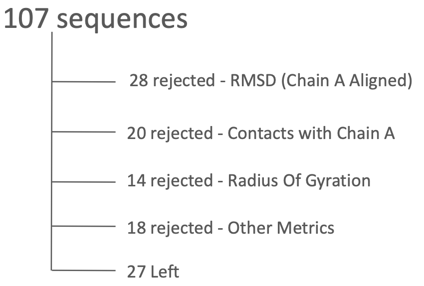
Filtering from 107 sequences to 27
The final filtering process removed candidates in several steps (Fig. 6):
· 28 were rejected by RMSD
· 20 were rejected by Chain A contact requirements
· 14 were rejected by radius of gyration
· 18 were rejected by other metrics
· 27 remained
As desired, the final group still contained structural variety. Looking at two examples, model A has a strongly beta-rich design that survived the full pipeline, while model B has a design with a more even mix of alpha and beta content (Table 2, Fig. 7).
The AlphaFold3 evaluation stage reduced 107 sequences to 27 final designs
These 27 candidates represented the final computational output of the summer project.
The 27 final binder designs that passed the computational pipeline
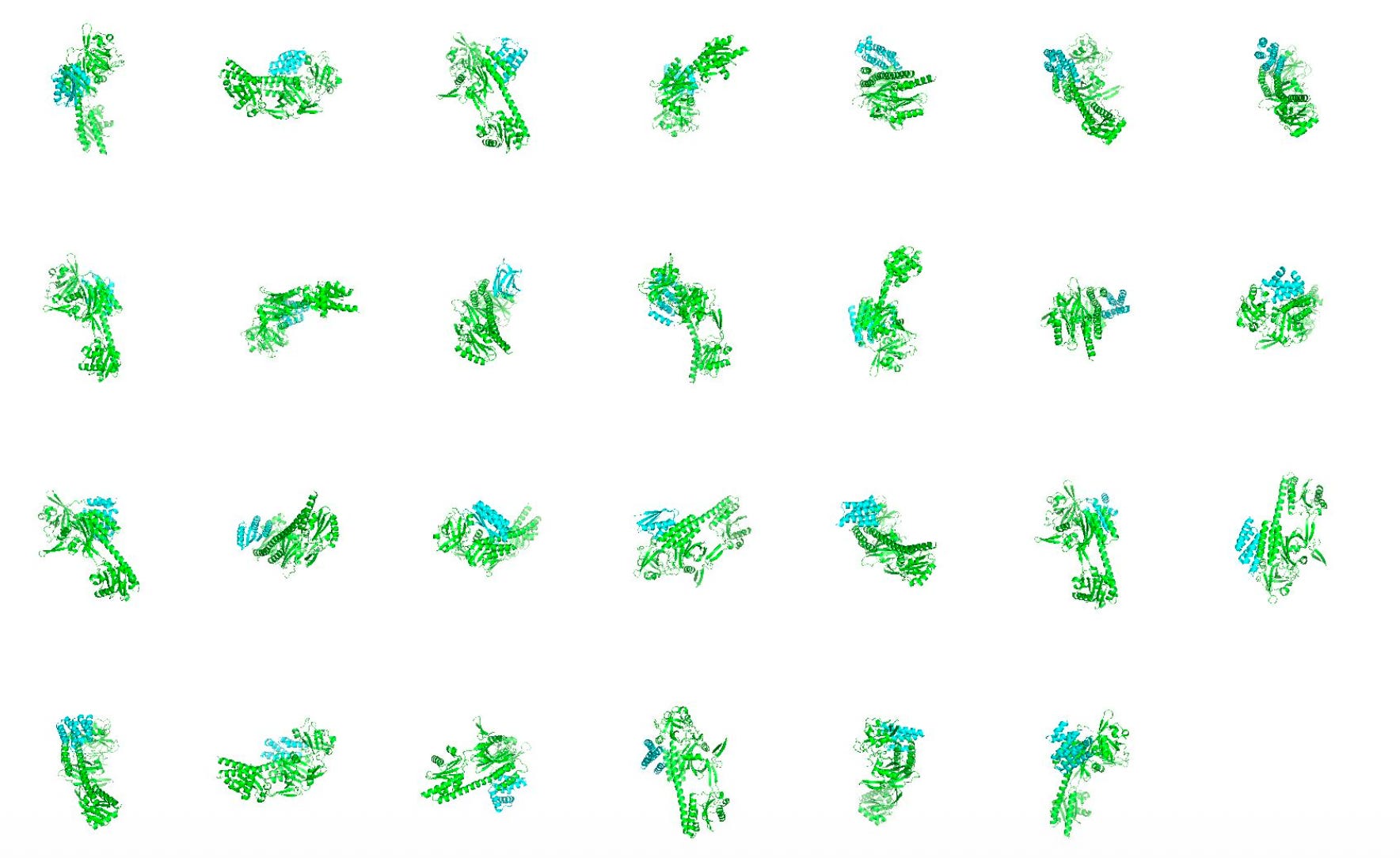
Examples of the final designs
The final group still contained structural variety.
One example binder had:
Length: 97
Radius of gyration: 12.515
Beta content: 78.35 percent
Loop content: 21.65 percent
RMSD: 4.97
dG/dSASA: negative 2.29
A second example had:
Length: 108
Radius of gyration: 12.23
Alpha content: 35.19 percent
Beta content: 39.81 percent
Loop content: 25 percent
RMSD: 5.03
dG/dSASA: negative 2.37
Two final candidates: one beta-rich design and one design with a more balanced alpha-beta structure
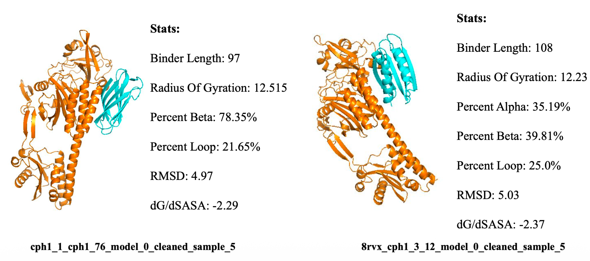
The first example shows that a strongly beta-rich design survived the full pipeline. The second shows a design with a more even mix of alpha and beta content.
Technical problems during the project
It is important to note that the pipeline did not run smoothly at every stage. One problem involved out-of-memory errors during RFdiffusion3. Future efforts should consider to increase the memory and time settings and change computing partitions. Additionally, FastRelax created another challenge. The original local FastRelax approach was applied late in the pipeline. According to the project summary, this led to candidate models loss, unwanted movement of Chain A, and restricted flexibility for the binder. In response, we changed the method by distributing global FastRelax across all 3,700 post-threaded models. The jobs were run with up to 500 jobs at one time. Chain A constraints were applied to maintain the target structure while allowing more binder flexibility. These problems showed that the computing workflow was not separate from the scientific work. Job settings, constraints, and pipeline order could affect which candidates survived.
What comes next
After this long process, these 27 candidates represented the final computational output of the summer project. These designs can now be submitted to experimental validation. The wet-lab results would provide information that the team could use to adjust later filtering choices.
In this sense, the team identified three future directions for the project:
1. Test the de novo binders in the wet lab
2. Increase the initial RFdiffusion3 backbone set from about 1,000 to 10,000
3. Improve the pipeline and filtering decisions using results from wet-lab testing
And so, I reach the end of this series of posts stemming from our my summer project!