Designing a Protein Binder: From Target Selection to Final Candidates - Part 3

Designing Sequences While Preserving Diversity

[In the summer of 2026, I had the opportunity to conduct research in the Khare Laboratory at Rutgers University under the mentorship of Dr. Sagar Khare and Austin Seamann. The Khare Lab is part of the Institute for Quantitative Biomedicine (IQB), and Dr. Khare is a Professor in the Department of Chemistry and Chemical Biology. My project focused on using AI-based protein design tools to design a binder for a photoswitchable protein. Below is a summary of the research, methods, and key outcomes from the project. ]

Previous in the series: Generating More Than 1,000 Binder Backbones

Moving from protein backbones to amino-acid sequences

In the previous post I explained how after RFdiffusion3 filtering, we came up with 370 proposed binder backbones. But what exactly is a backbone? A backbone describes the overall shape of a protein, but it does not fully define the amino-acid sequence that should form that structure. In this next stage, we used ProteinMPNN to design those sequences. The goal was not only to produce strong candidates, but also to avoid ending with a final group of binders that all looked or interacted in the same way.

Designing only the binder sequence

While the Cph1 target was Chain A, we treated the new binder as Chain B in this part of the workflow. We asked ProteinMPNN to design only the sequence of the binder; however, we still gave the model structural context from Chain A (Fig. 1). This was an important step in our workflow because the sequence at the binder interface should respond to the residues on the target. The transcript gives the example that if a residue on Chain A is hydrophobic and contacts the binder, the designed binder residue may also need a compatible property. For each of the 370 backbones, ProteinMPNN generated 10 sequences, producing a total of 3,700 sequences.

ProteinMPNN designed the binder sequence while using Chain A as structural context

caption...

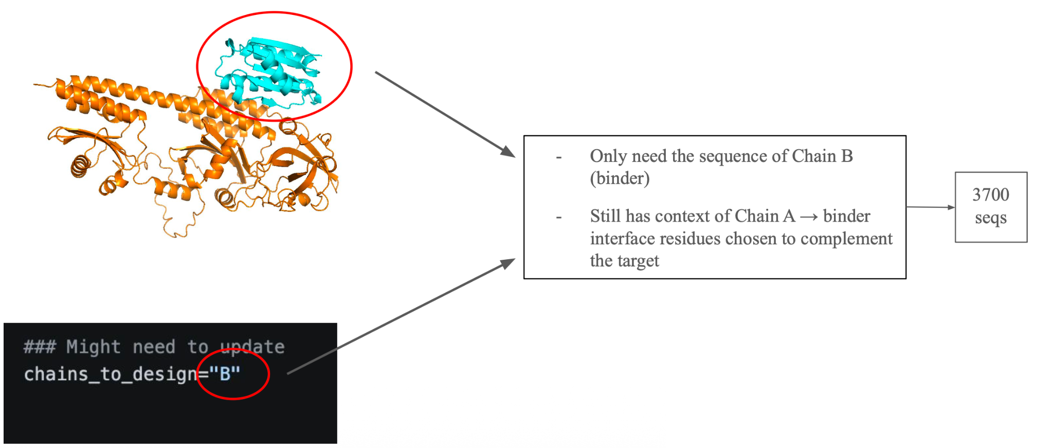
For each of the 370 backbones, ProteinMPNN generated 10 sequences. This produced a total of 3,700 sequences.

Threading and FastRelax

After obtaining these new sequences, we processed them with threading and FastRelax. Threading placed each designed amino-acid sequence onto its RFdiffusion3 backbone. Then, FastRelax adjusted the side chains and backbone (Fig. 2). The purpose of this process was to refine the structure and move it into a more relaxed arrangement, although the changes were sometimes small. In the examples, the threading and FastRelax output mostly overlap, but the helices and nearby regions do not match perfectly. After this stage, we had 3,700 refined structural models, with proper amino-acid sequences.

FastRelax made local adjustments to the threaded structures

Figure 2

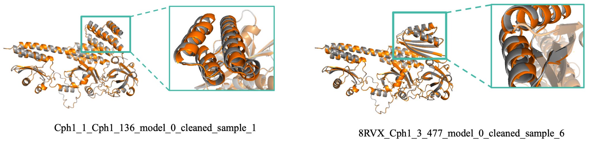
After this stage, we had 3,700 refined structural models.

Filtering by interface energy

At this stage, we added a new, relevant, metric: dG/dSASA. In the overall project, I described this metric as interface binding energy divided by the amount of surface area involved in binding. The key point was that more negative values were treated as more favorable (Fig. 3). Across the full set, most values fell between -1 and -3. For alpha-rich designs, we used a cutoff below -2.35. For beta-rich designs, we later used a looser cutoff below -1.80.

The dG/dSASA distribution used to prioritize designs by interface energy

Figure 3

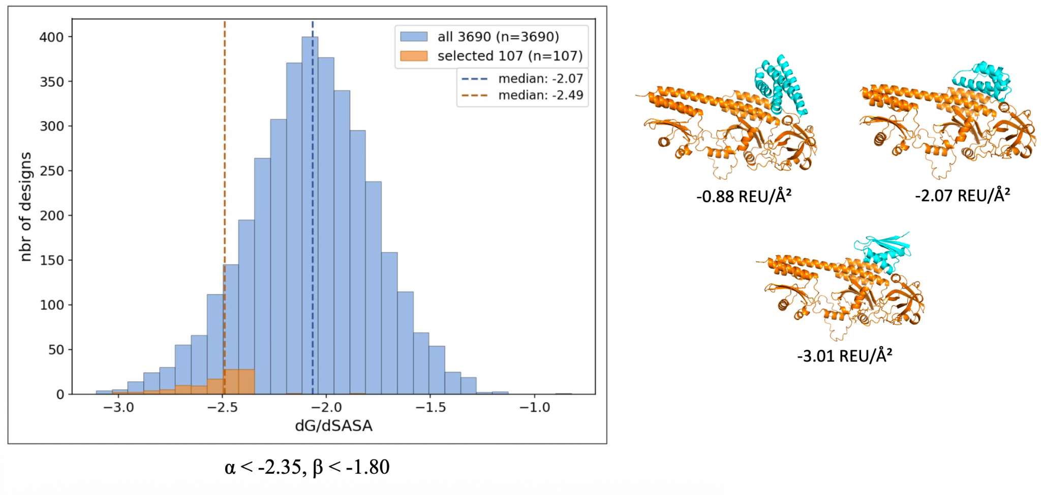
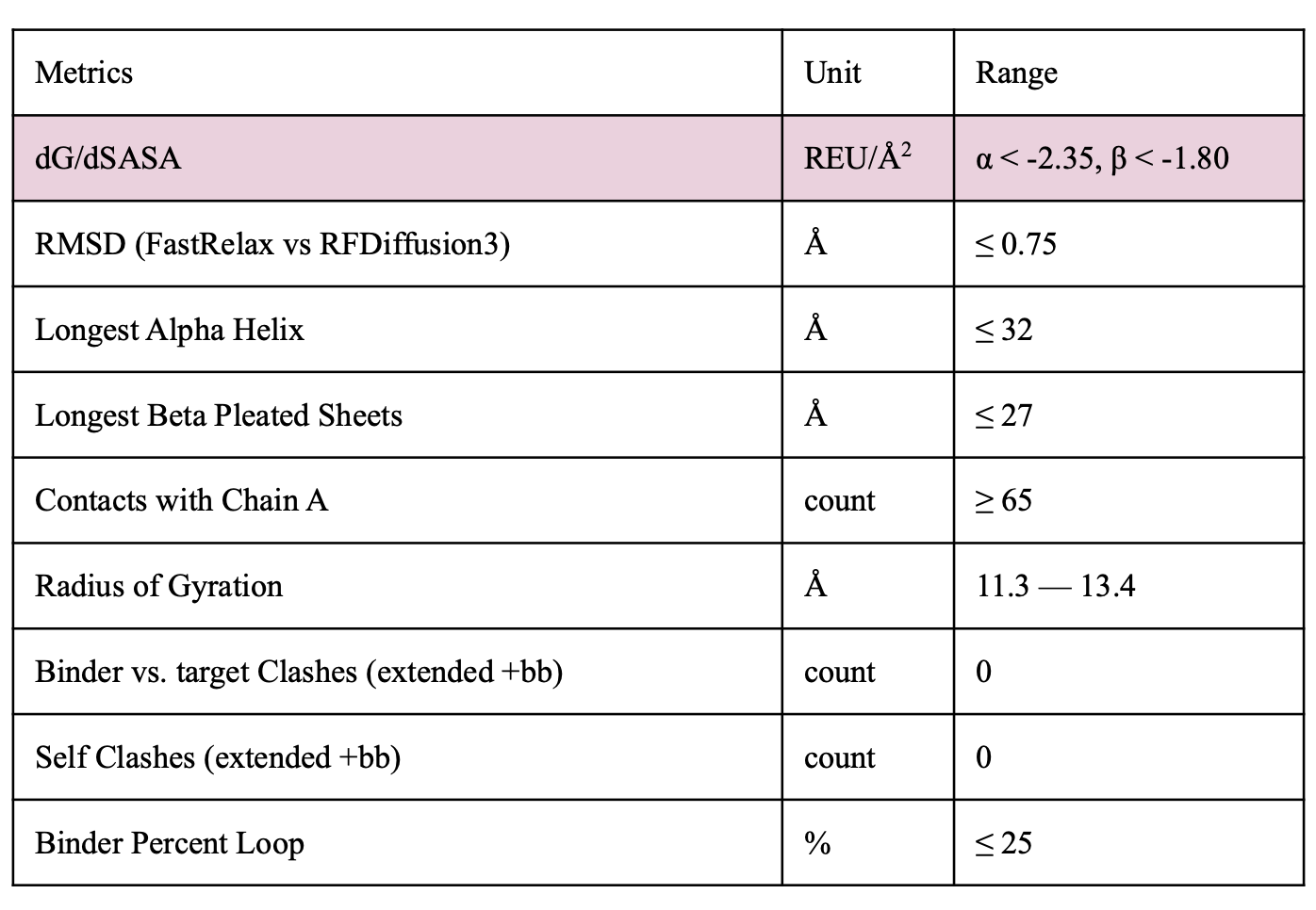
We also measured the root mean square deviation (RMSD) between the FastRelax output and the earlier RFdiffusion3 structure. The cutoff table for this stage used an RMSD of 0.75 angstroms or less. As previously stated, we included other filters, such as contacts with Chain A, radius of gyration, loop percentage, clashes, and the maximum lengths of helices and beta sheets (Fig. 4).

The post-ProteinMPNN metric ranges used to filter the 3,700 designs

Figure 4

A bias toward alpha-helical designs

One thing that we noticed as we reviewed the candidate models was that RFdiffusion3 strongly favored helical structures. After applying strict cutoffs, many beta-rich designs were removed, and this created a problem for our goal of maintaining diversity. If every final binder had a similar alpha-helical structure, the final set would test only a narrow region of the available design space. To address this issue, we created a beta rescue. We allowed designs with more than 70% beta content to use a less strict dG/dSASA cutoff. Instead of requiring a value below -2.35, they needed a value below -1.80 (Fig. 5). This did not mean that all beta-rich designs automatically passed, but it constituted a different threshold so that some of those designs could remain in the candidate set.

A looser interface-energy cutoff helped protect beta-rich designs from the pipeline’s helix bias

Figure 5

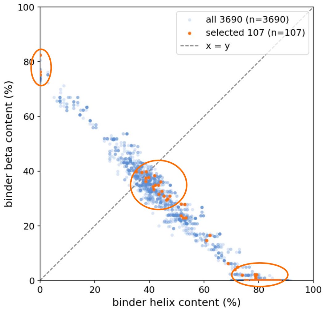
This did not mean that all beta-rich designs automatically passed. It gave them a different threshold so that some could remain in the candidate set.

Preserving different structural types

Our selected designs included different combinations of alpha helices and beta sheets.

One example had:

• 0 percent alpha

• 82.52 percent beta

A second had:

• 38.78 percent alpha

• 39.8 percent beta

A third had:

• 85.86 percent alpha

• 0 percent beta

Selected binders included beta-rich, mixed alpha-beta, and alpha-rich structures

Figure 6

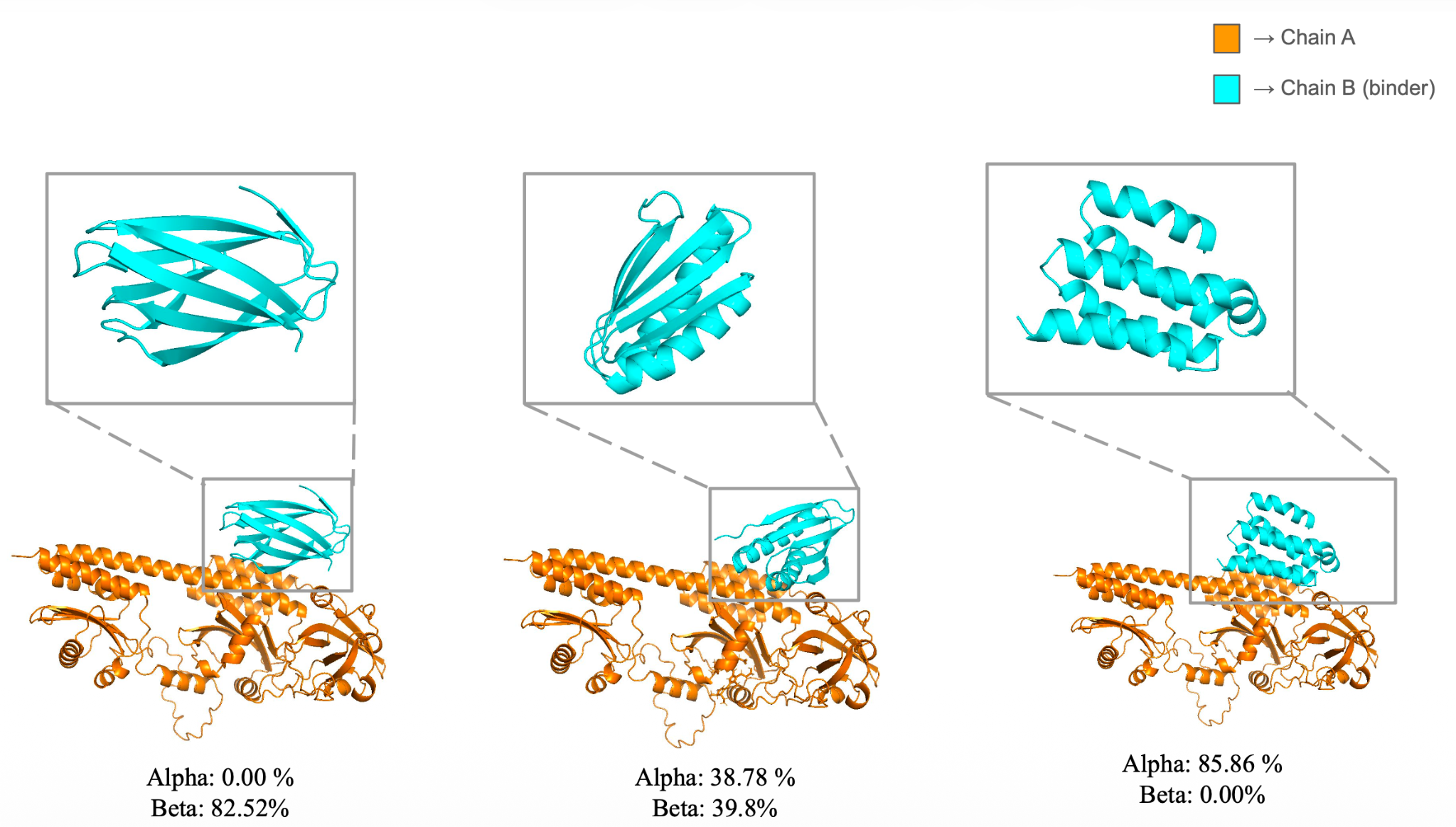
These structures looked very different from one another. That variety was intentional.

The team wanted the final designs to represent several possible structural solutions rather than repeating the same type of binder.

Preserving different binding poses

We also wanted the binders to occupy different positions near the target interface.

A binder’s pose describes where it sits against the target. If all designs used the same pose and that region later failed in the wet lab, then many candidates could fail for the same reason.

To estimate pose diversity, we compared the proposed binder with the position of Chain B in the Cph1 dimer.

A lower number of clashes meant that the binder tended to sit farther from the original dimeric interface. A higher number meant that the binder extended more deeply into that space.

Different overlap values with the original Cph1 Chain B position were used to preserve binder-pose diversity

Figure 7

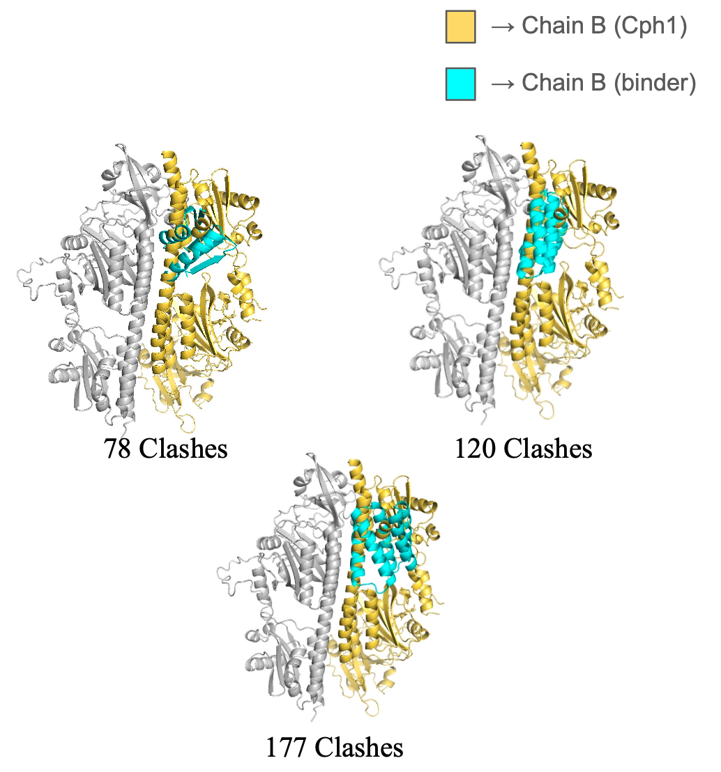
This gave us a way to retain designs that approached the target from different positions.

Reducing 3,700 designs to 107

The above-mentioned filters greatly reduced the candidate set (Fig. 8). The largest change came from the dG/dSASA filter. The later filters removed additional candidates based on structural agreement, contact quality, compactness, secondary structure, and clashes. The slide lists the progression as follows:

· 3,700 designs started the stage

· dG/dSASA removed 3,256

· RMSD removed 115

· Percent loop removed 110

· Chain A contacts removed 38

· Radius of gyration removed 19

· Helix and sheet length removed 43

· Self-clashes removed 2

· 107 designs remained

Post-ProteinMPNN filtering reduced 3,700 sequence-based designs to 107

Figure 8

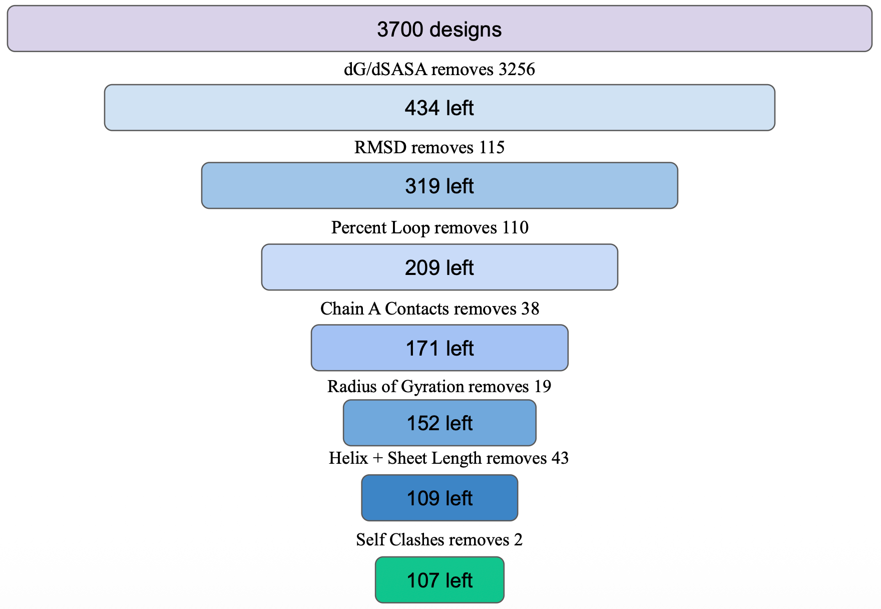
The largest change came from the dG/dSASA filter. The later filters removed additional candidates based on structural agreement, contact quality, compactness, secondary structure, and clashes.

Conclusion

ProteinMPNN expanded 370 backbones into 3,700 possible sequences. Threading and FastRelax then created refined structures for those sequences.

Our filters reduced the set to 107 designs. During this process, we also made a deliberate choice to protect diversity. We kept different secondary-structure types and different binding poses so that the final candidates would not all depend on the same structural idea.

The remaining 107 sequences then moved into AlphaFold3 for the last major computational evaluation.

Next in the series: How AlphaFold3 predictions and final metrics reduced 107 sequences to 27 candidates for possible wet-lab testing.