

[In the summer of 2026, I had the opportunity to conduct research in the Khare Laboratory at Rutgers University under the mentorship of Dr. Sagar Khare and Austin Seamann Ph.D. Stud. The Khare Lab is part of the Institute for Quantitative Biomedicine (IQB), and Dr. Khare is a Professor in the Department of Chemistry and Chemical Biology. My project focused on using AI-based protein design tools to design a binder for a photoswitchable protein. Below is a summary of the research, methods, and key outcomes from the project. ]
Previous in the series: Choosing the Target and Building the Protein-Design Pipeline
Using RFdiffusion3 to create and filter de novo structures
On our previous post I explain how we selected the binding region on Cph1; now here I will explain the process by which we generated possible binder structures. To achieve this, I used RFdiffusion3, a generative AI model that creates new protein backbones for a target site. These backbones were de novo designs, meaning that the model didn’t simply modify existing binders, but rather created new structural shapes based on the target and hotspot information we provided.
Testing the amount of target context and running RFdiffusion3 at scale
Before running the model at full scale, we needed to answer an important setup question: How much of the Cph1 structure should RFdiffusion3 see? This is important because if we provided the program a large portion of the protein, the simulations would be more precise, but the computing power required could be very high. On the other hand, if we provided it a minor portion, the computing requirements would lower, but at risk of delivering inadequate models. We decided to compare three levels of structural context (Fig. 1): the first option included 160 selected residues, the second included 249 residues, and the final option included the full 492-residue Cph1 monomer.
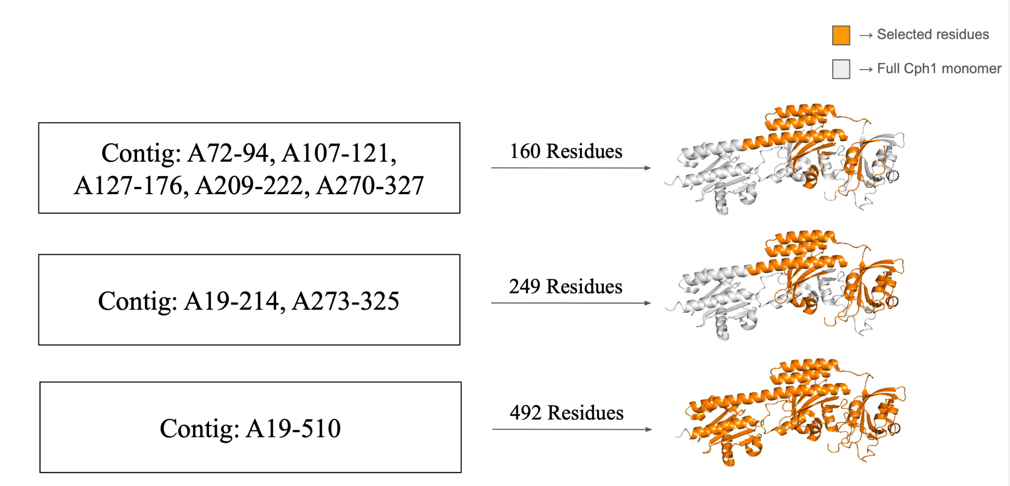
After comparing the test process and the preliminary results, we selected the complete 492-residue monomer, based on two main reasons. First, using the full monomer rarely caused GPU out-of-memory errors during the initial testing. Second, the complete protein gave RFdiffusion3 the greatest amount of structural context while it designed binders around the target region. The final contig was listed as A19–510.
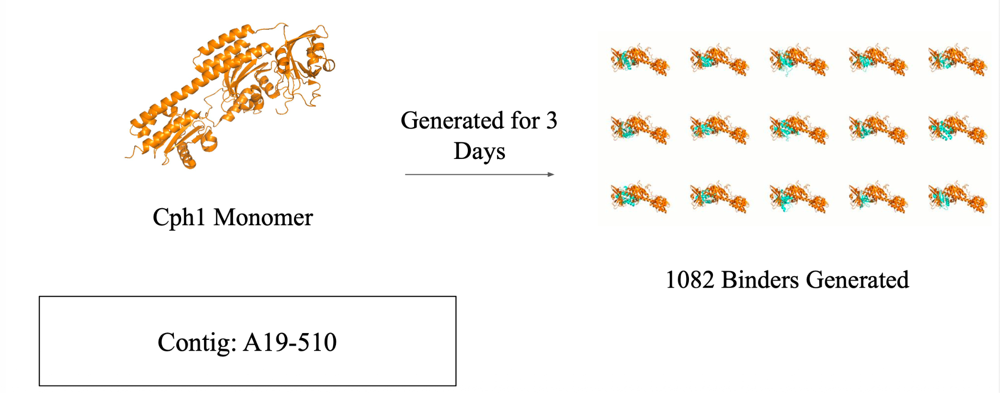
The proper binder backbones generation took about three days. The transcript notes that the run was slower than expected because of summer heat waves and unavailable computing nodes, aspects that we will take into consideration in future projects. At the end of the run, RFdiffusion3 had generated 1,082 binder backbones. After this, our next step was coming up with a consistent way to remove structures that appeared unrealistic or poorly suited to the target.
Building the first structural filter
We evaluated the RFdiffusion3 outputs using several metrics, each addressing a different feature of the proposed binder (Fig. 2):
· Radius of gyration
· Clashes with Chain A
· Self-backbone clashes within the binder
· Loop percentage
· Clashes with the dimeric Chain B position
· Length of the longest alpha helix
· Length of the longest beta sheet
· Minimum number of contacts with Chain A
We will now explain some of these metrics with more detail.
Using the full Cph1 monomer, RFdiffusion3 generated 1,082 binder backbones over about three days
Selecting compact structures
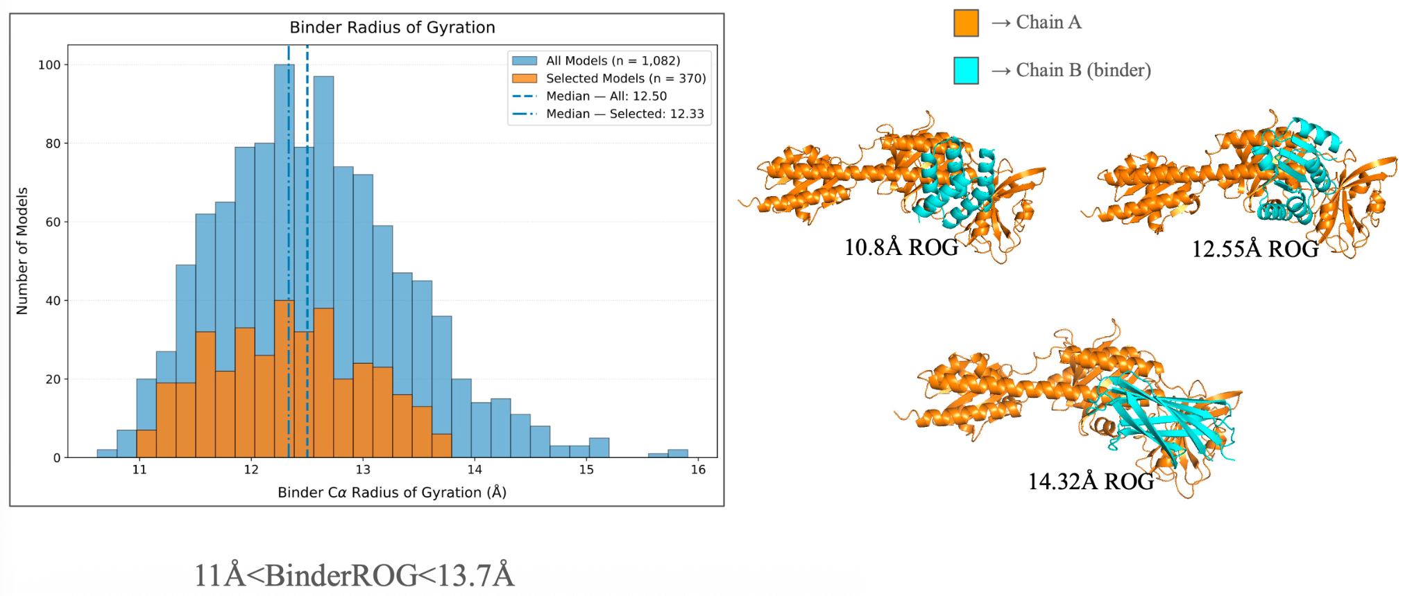
The first step into selecting which binder models could be adequate for experimental testing was measuring the radius of gyration. This is a measure that describes the distribution of the atoms of a protein around its center of mass. In other words, it measures how compact each binder was. Very small values could represent an unrealistically collapsed structure, whereas larger values could represent an extended structure that might not fold or interact as intended. We kept binders with a radius of gyration between 11 and 13.7 angstroms. This range was selected by looking at the distribution of generated binders and visually reviewing example structures (Fig. 4).
The structural metrics and initial cutoff ranges used to filter RFdiffusion3 outputs
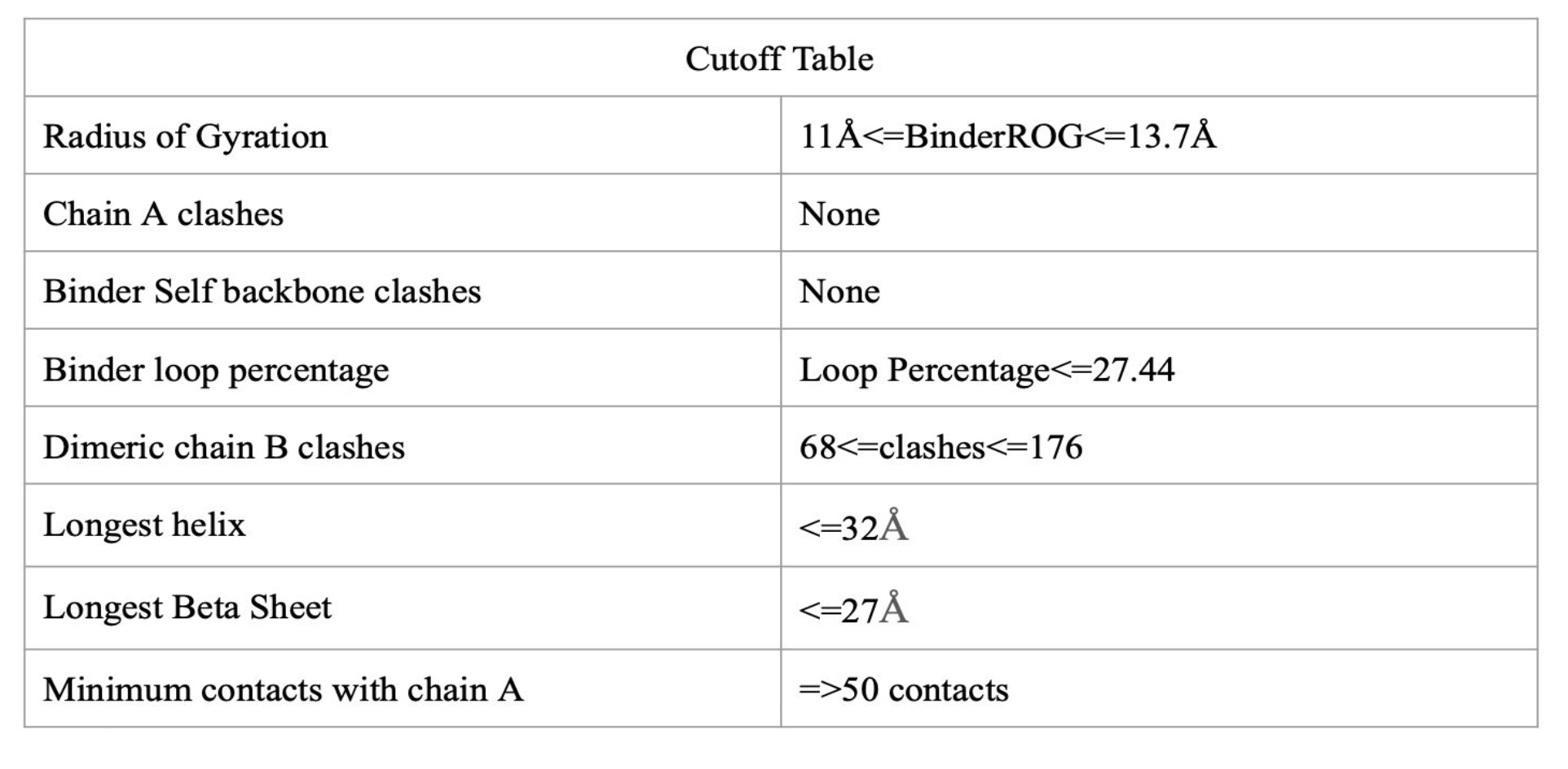
Each metric addressed a different feature of the proposed binder.
Selecting compact structures
Radius of gyration measured how compact the binder was.
Very small values could represent an unrealistically collapsed structure. Larger values could represent an extended structure that might not fold or interact as intended.
We kept binders with a radius of gyration between 11 and 13.7 angstroms. This range was selected by looking at the distribution of generated binders and visually reviewing example structures.
Radius-of-gyration filtering favored compact binders between 11 and 13.7 angstroms
Limiting flexible loop content
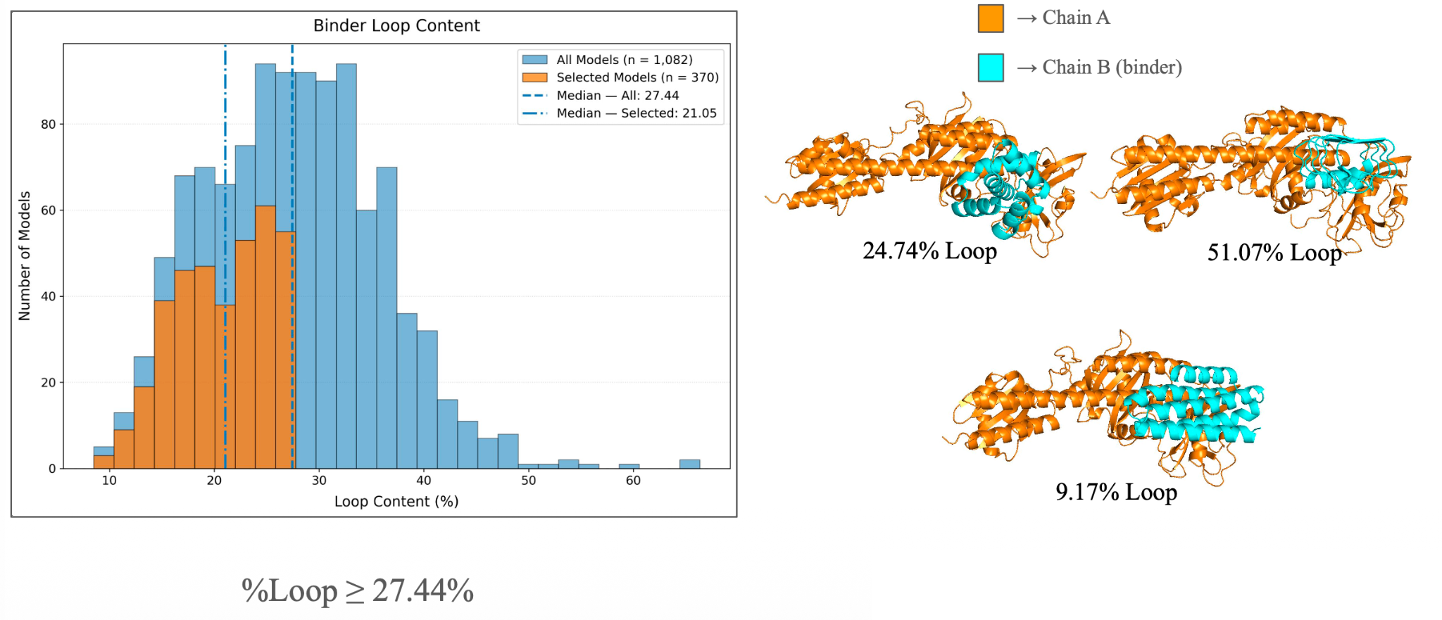
We also measured the percentage of how much each binder was made up of loops. In our filtering approach, binders with unusually high loop content were less desirable. We decided this because loops were treated as more flexible than alpha helices and beta sheets, so designs with too much loop content could be harder to design reliably. The cutoff table set binder loop percentage at 27.44% or less (Fig. 5).
Examples of binders with different loop percentages used to guide the loop-content filter
Restricting oversized structural elements
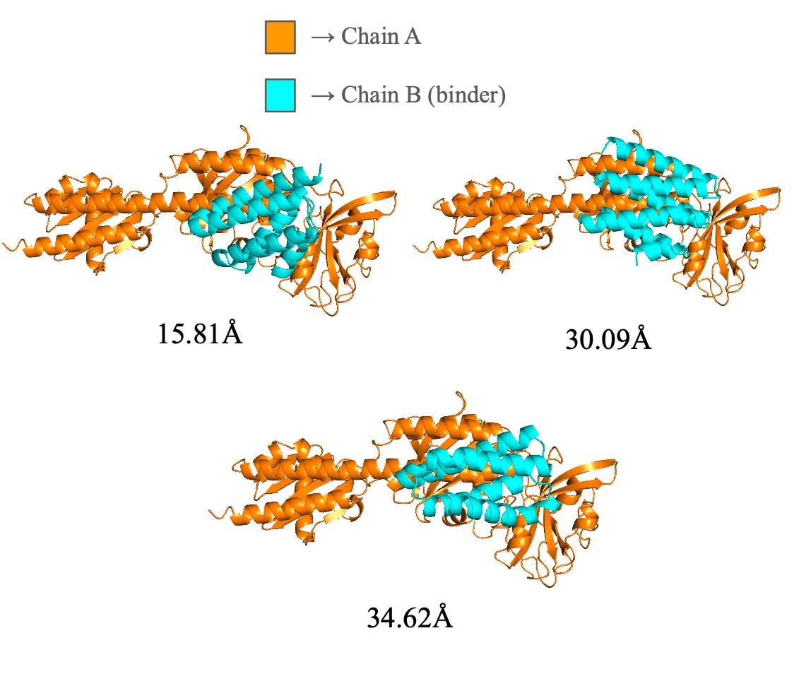
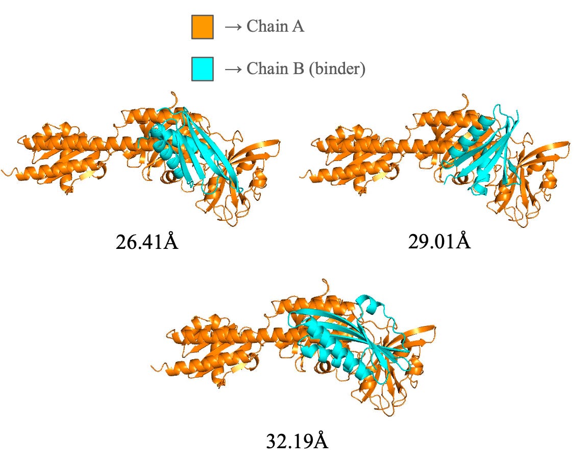
Other filter metrics that we used were the length of the longest alpha helix and the longest beta sheet. On one side, very long helices could create elongated structures that were not preferred for this target. On the other side, large beta sheets could dominate the fold and create broad or flat interfaces. We defined the alpha-helix and longest beta sheet limits as 32 and 27 angstroms, respectively (Fig. 6, Fig. 7). Some structures shown as selected in the original histograms extended past these helix and sheet limits. The transcript explains that these two cutoffs were not applied during the first RFdiffusion3 filtering run. They were added later, after the ProteinMPNN stage.
The longest alpha helix was limited to 32 angstroms
The longest beta sheet was limited to 27 angstroms
Filtering overview
The filtering pipeline described above reduced the 1,082 RFdiffusion3 binders to 370 candidates. The largest listed reduction came from loop content. Radius of gyration, backbone clashes, and contact requirements removed additional structures. The total number of models rejected per each metric was as follows:
· 130 rejected because of backbone clashes
· 104 rejected because of contact criteria
· 358 rejected because of loop percentage
· 120 rejected because of radius of gyration
· 370 passed the filtering stage
The remaining 370 candidate models had designed shapes, but they did not yet have the final amino-acid sequences needed for the next stages of the project.
The first filtering stage reduced 1,082 RFdiffusion3 binders to 370 candidates
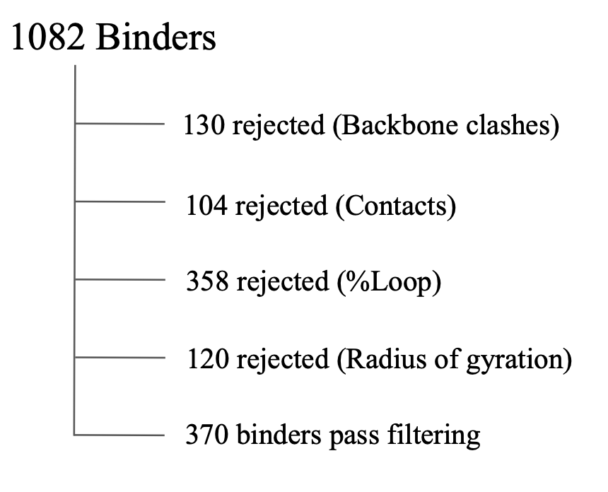
The largest listed reduction came from loop content. Radius of gyration, backbone clashes, and contact requirements removed additional structures.
These 370 candidates then moved into the next major stage: sequence design.
Conclusion
RFdiffusion3 gave us a large starting set of possible binder backbones. We selected the full Cph1 monomer as input because it provided the greatest structural context and remained workable on the available GPUs.
The model produced 1,082 designs. By filtering for compactness, loop content, structural-element length, contacts, and clashes, we reduced that set to 370 candidates.
Those candidates had designed shapes, but they did not yet have the final amino-acid sequences needed for the next stages of the project.
Next in the series: How we used ProteinMPNN and FastRelax to generate 3,700 sequence-based designs while preserving structural and positional diversity.